FX's Projects
Musings involving electronics, systems, and stuff hackers care about.
CORDIC optimization for an FPGA
Another recent one, this time mainly in verilog. The main algorithm code is inline below, but I have a more comprehensive repo with testbenches and an integration in this github repo. I can make it available to you on a limited basis if you contact me on my LinkedIn.
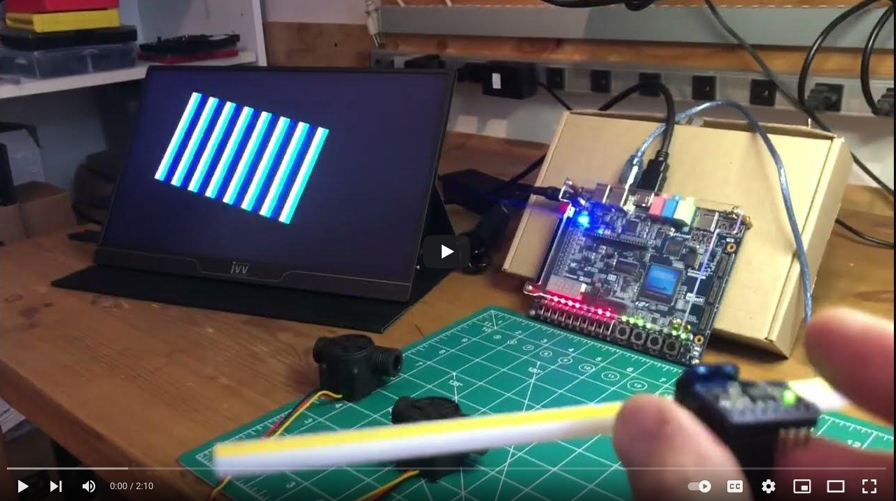
As discussed in the ESP32 Flow and Temperature Project project, an IMU platform is used to rotate an image on an hdmi screen. The bar graphs displayed on the hdmi screen can be dynamically rotated by an angle coming from the roll of the IMU platform.
flowchart LR
    %% Nodes
    A[IMU \n Platform]
    B[CORDIC \n Module]
    C[HDMI \n Module]
    E[Rotated \n Bar \n Graphs]

    %% Connections
    A -->| Roll \n angle | B
    B -->| sin \n cos | C
    C -->| Rotation \n matrix | E
The angle of the roll is fed into a cordic module to compute separate sin and cos values. These values are then fed into the hdmi module to prepare a rotation matrix used to properly rotate the pixels to display.
The CORDIC - (COordinate Rotation DIgital Computer) algorithm was selected for the task of finding the cos and sin of an angle because it is an interesting case of very efficient mathematical optimisation. It is usually found as an iterative process that is very well suited for FPGA implementation in a FSM (Finite State Machine) using only additions and bit shifts to replace multiplication. The algorithm is very efficient in that very few resources are used and that they run fast. The specific implementation can be tuned to reach high precision when required. We typically reach a precision of 0.0001 or better with the code presented here.
The idea here is to first describe the basic mathematical optimization. A fixed point implementation is shown next with accompanying verilog.
Inspiration
The material is inspired from an excellent in depth blog as found on All about circuits on the introduction to the cordic algorithm extending it here with a verilog implementation.
For the astute reader that would like even more in depths details, there is a also this article, published in 2009 for the 50 years of the invention of the algorithm by Jack E. Volder. This IEEE paper here is a must read if you want to learn about the other modes of operation of the algorithm that yield polar to rectangular conversions, hyperbolic functions, division and many more.
Algorithm overview
The algorithm, as implemented, takes an angle as an input and will output the sin and cos components associated with this angle. One remembers that, on the unit circle, sin represents the vertical component of the rotated vector while cos represents its horizontal component.
The concept of the algorithm is to iteratively rotate a vector using a set of known rotation angles until a good match is reached with the input angle. Each successive rotation is smaller than the previous and modifies the x and y components values of the rotating vector until the desired precision is reached. In our case, the iteration number is 16, regardless of the precision reached, as simulation has proven a known performance for all input values.
The rotation mechanics is such that a starting point $(x_0, y_0)$ representing our rotating vector on the unit circle is rotated by $\theta$ to the point $(x_1, y_1)$ by:
\[\begin{equation} \begin{aligned} x_1 = x_0 \cos{\theta} - y_0 \sin{\theta} \\ y_1 = x_0 \sin{\theta} + y_0 \cos{\theta} \end{aligned} \end{equation}\]Or, in matrix form:
\[\begin{equation} \begin{bmatrix} x_1 \\ y_1 \\ \end{bmatrix} = \begin{bmatrix} \cos{\theta} & -\sin{\theta} \\ \sin{\theta} & \cos{\theta} \end{bmatrix} \begin{bmatrix} x_0 \\ y_0 \end{bmatrix} \end{equation}\]Starting with a vector $(x_0, y_0) = (1,0)$ along the x axis, we could use eq.2 to find the desired components $x_1$ and $y_1$ of the rotated vector by an angle of $\theta$, yielding the required output of $\cos{\theta}$ and $\sin{\theta}$. However this, in a weird circular reference, requires that both $\cos{\theta}$ and $\sin{\theta}$ be computed… We will have to work this out carefully to find a proper form that is both precise and efficient to compute with the hardware present in an FPGA.
The path to optimization
We have to get rid of costly multiplications. Let’s consider an iterative approach. The first order of business is to accept that we can reconstruct any rotation angle by summing or subtracting known rotation angles that are carefully selected. In other words, we can always superpose our constructed vector on top of the desired one given 16 attempts at rotating it by picking into a set of precomputed angles.
To help picture these sequential rotations, we can compose transformations based off of eq.2. Let’s factor out $\cos{\theta_1}$ to represent one rotation.
\[\begin{equation} \begin{bmatrix} x_1 \\ y_1 \end{bmatrix} = \cos{\theta_1} \begin{bmatrix} 1 & \tan(\theta_1) \\ -\tan(\theta_1) & 1 \end{bmatrix} \begin{bmatrix} x_0 \\ y_0 \end{bmatrix} \end{equation}\]Combining two rotations yields:
\[\begin{equation} \begin{bmatrix} x_2 \\ y_2 \end{bmatrix} = \cos{\theta_2} \begin{bmatrix} 1 & \tan(\theta_2) \\ -\tan(\theta_2) & 1 \end{bmatrix} \cdot \cos{\theta_1} \begin{bmatrix} 1 & \tan(\theta_1) \\ -\tan(\theta_1) & 1 \end{bmatrix} \begin{bmatrix} x_0 \\ y_0 \end{bmatrix} \end{equation}\]Which, by grouping the terms and generalizing for n step rotations:
\[\begin{equation} \begin{bmatrix} x_n \\ y_n \end{bmatrix} = \prod_{i=0}^{n-1} \cos{\theta_i} \cdot \prod_{i=0}^{n-1} \begin{bmatrix} 1 & \tan(\theta_i) \\ -\tan(\theta_i) & 1 \end{bmatrix} \cdot \begin{bmatrix} x_0 \\ y_0 \end{bmatrix} \end{equation}\]This representation, while a bit more challenging to decode, yields a few interesting properties. First, as $\cos{\theta}$ is a pair function, it will stay positive for angles within $[-\frac{\pi}{2}, \frac{\pi}{2}]$. Then, since we are using smaller angles, $cos$ approaches 1 and in the algorithm, the product converges towards a constant number $K_{fixed} \approxeq 0.6072$.
Similarly, and since $cos$ is pair while $sin$ is odd in the considered domain, we infer that $\tan$ will be odd. All this to say that the sign of the angle can be factored out and the equation eq.6 really is:
\[\begin{equation} \begin{bmatrix} x_n \\ y_n \end{bmatrix} = K_{fixed} \cdot \prod_{i=0}^{n-1} \begin{bmatrix} 1 & \sigma \cdot \tan(\theta_i) \\ -\sigma \cdot \tan(\theta_i) & 1 \end{bmatrix} \cdot \begin{bmatrix} x_0 \\ y_0 \end{bmatrix} \end{equation}\]With $\sigma$ taking the value +1 for counterclockwise rotation and -1 for clockwise rotations while $\theta_i$ remains always positive.
So, we got rid of some complexity, at the expense of a scaling factor $K_{fixed}$. Since we have to start the algorithm with a vector of length one as the first vector to be rotated, we can premultiply this vector by a constant. All that is involved is to set $(x_0, y_0) = (K_{fixed}, 0)=(0.6072, 0)$ and the multiplying factor is now baked into the algorithm.
Let’s now look into the remaining operations. We are left with a constant $K_{fixed}$ that scales a matrix product with 16 iterations. In these matrices the $\theta_i$ are known in advance and selected for very specific properties. Let’s consider a favorable case with angles chosen so that:
\[\tan(\theta_i) = 2^{-i}\]No more conventional multiplications
This choice leads to two very important consequences. The first consequence of the angle selection is that the matrices all become very easy to implement, taking n=16 as an example and all positive angle rotations:
\[\begin{equation} \prod_{i=0}^{n-1} \begin{bmatrix} 1 & \tan(\theta_i) \\ -\tan(\theta_i) & 1 \end{bmatrix} = \begin{bmatrix} 1 & 2^{0} \\ -2^{0} & 1 \end{bmatrix} \begin{bmatrix} 1 & 2^{-1} \\ -2^{-1} & 1 \end{bmatrix} \begin{bmatrix} 1 & 2^{-2} \\ -2^{-2} & 1 \end{bmatrix} \ldots \begin{bmatrix} 1 & 2^{-15} \\ -2^{-15} & 1 \end{bmatrix} \end{equation}\]We effectively transformed the matrices into multiplications by powers of 2 and, as you may have anticipated, these are equivalent to very simple and efficient bit shifts. All of the operations required within the $\prod$ are now signed additions or sign extended bit shifts. These happen to map very efficiently to hardware ressources in an FPGA. No more conventional multiplications whatsoever.
Sign selection process
Let’s take a closer look at the signs of the angles. We just presented a case with the product of 16 rotation steps with positive $\theta_i$.
Talking about the angles, the second consequence of their specific selection is that these $\theta_i$ are all precomputed and equal to $\theta_i = \arctan(2^{-i})$. This yields a series of 16 progressively smaller angle increments at our disposal that converge to be about half of the preceding one. The first angle is $\frac{\pi}{4}$, the last angle being $\arctan(2^{-15}) \approxeq 0.00003$, or less than $0.002 ^\circ$.
Selectively adding or subtracting these angles can lead to reconstruct just about any angle between $[-\frac{\pi}{2}, \frac{\pi}{2}]$ to within $0.00003$ rad.
Putting it all together
So, on one side we have a very easy to compute rotation matrix using any of the $\tan(\theta_i)$ values, and on the other side we have very specific angles that we know in advance and that are associated with each and every easy to compute rotation matrix.
The last part of the puzzle to understand the CORDIC algorithm is to recognize that by carefully selecting the sign of these 16 rotations, one can reconstruct on the fly just about any angle in the range. And the algorithm does just about that: step rotations are performed starting with the bigger angles and through to the smallest. The x and y components of the rotated output vector are summed up at each step, representing the cos and sin of the internal vector chasing the requested angle.
The real kicker is that the algorithm will just pick the next rotation as either a positive or a negative one and so that the vector would end up closest to the desired angle after the 16 rotations. This is a feedback loop of sorts that uses imposed angles but decides if it should add or subtract the angle to its own advantage in the goal of ending on the required final angle.
The result is that the 16 rotations will bring the reconstructed angle of the internal vector closer to the desired angle until they match to within the precision required. The components at that moment, the x and y values, are the cos and sin of the reconstructed angle and very closely match the ones for the requested angle.
Fixed point math
A small note here on the fact that the algorithm and all internal constants are prescaled by a factor $2^{15}$ or $32768$ since most of the internal computations represent values not much larger than 1 in absolute value. In the code, arbitrary register width can be used as long as the ressources are available.
Verilog code
Here is the verilog code to implement the algorithm.
1
2
3
4
5
6
7
8
9
10
11
12
13
14
15
16
17
18
19
20
21
22
23
24
25
26
27
28
29
30
31
32
33
34
35
36
37
38
39
40
41
42
43
44
45
46
47
48
49
50
51
52
53
54
55
56
57
58
59
60
61
62
63
64
65
66
67
68
69
70
71
72
73
74
75
76
77
78
79
80
81
82
83
84
85
86
87
88
89
90
91
92
93
module cordic #(
// Internal parameters and signals
parameter INTERNAL_WIDTH = 17,
parameter IO_WIDTH = 17,
parameter ITERS = 16,
parameter PREFIX = 15,

    parameter [INTERNAL_WIDTH-1:0] K_FIXED =
        (PREFIX == 15) ? {INTERNAL_WIDTH{1'b0}} | 15'sh4dba :
        (PREFIX == 16) ? {INTERNAL_WIDTH{1'b0}} | 16'sh9b75 :
        (PREFIX == 17) ? {INTERNAL_WIDTH{1'b0}} | 17'sh136ea :
        {INTERNAL_WIDTH{1'b0}} // Default value if PREFIX does not match

)(
input wire clk,
input wire reset,
input wire signed [IO_WIDTH-1:0] angle_in,// Angle in fixed-point format
output reg signed [IO_WIDTH-1:0] cos_out, // Cosine output in fixed-point
output reg signed [IO_WIDTH-1:0] sin_out, // Sine output in fixed-point
output reg ready // Data ready signal
);

    reg signed [INTERNAL_WIDTH-1:0] x, y, alpha, theta;
    reg [4:0] step;                     // Iteration step counter
    reg running;                        // Indicates if the computation is in progress

    // Precomputed arctangent values (in fixed-point format, scaled by 2^16)
    reg [15:0] atan_table [0:15];
    initial begin
        atan_table[ 0] = 16'h6488; // atan(2^-0) * 2^15
        atan_table[ 1] = 16'h3b59; // atan(2^-1) * 2^15
        atan_table[ 2] = 16'h1f5b; // atan(2^-2) * 2^15
        atan_table[ 3] = 16'h0feb; // atan(2^-3) * 2^15
        atan_table[ 4] = 16'h07fd; // atan(2^-4) * 2^15
        atan_table[ 5] = 16'h0400; // atan(2^-5) * 2^15
        atan_table[ 6] = 16'h0200; // atan(2^-6) * 2^15
        atan_table[ 7] = 16'h0100; // atan(2^-7) * 2^15
        atan_table[ 8] = 16'h0080; // atan(2^-8) * 2^15
        atan_table[ 9] = 16'h0040; // atan(2^-9) * 2^15
        atan_table[10] = 16'h0020; // atan(2^-10) * 2^15
        atan_table[11] = 16'h0010; // atan(2^-11) * 2^15
        atan_table[12] = 16'h0008; // atan(2^-12) * 2^15
        atan_table[13] = 16'h0004; // atan(2^-13) * 2^15
        atan_table[14] = 16'h0002; // atan(2^-14) * 2^15
        atan_table[15] = 16'h0001; // atan(2^-15) * 2^15
    end

    always @(posedge clk or posedge reset) begin
        if (reset) begin
            // Reset all registers and signals
            x <= 0;
            y <= 0;
            theta <= 0;
            alpha <= 0;
            step <= 0;
            running <= 0;
            ready <= 0;
            cos_out <= 0;
            sin_out <= 0;
        end else if (!running) begin
                x <= K_FIXED;     // Premult by K_FIXED, the CORDIC gain
                y <= 0;
                theta <= 0;
                alpha <= angle_in;  // Load the input angle with sign extension
                step <= 0;
                running <= 1;
                ready <= 0;
        end else if (running) begin
            // Perform CORDIC iteration
            if (step < (ITERS-1)) begin       // 0 indexed
                // Compute sigma and update coordinates
                if (theta < alpha) begin
                    // sigma = +1
                    theta <= theta + atan_table[step];
                    x <= x - (y >>> step);    // x - y / 2^step, CCW rotation matrix approx.
                    y <= y + (x >>> step);    // y + x / 2^step, CCW
                end else begin
                    // sigma = -1
                    theta <= theta - atan_table[step];
                    x <= x + (y >>> step);    // x + y / 2^step, CW
                    y <= y - (x >>> step);    // y - x / 2^step, CW
                end
                step <= step + 5'sh01;
            end else begin
                cos_out <= x;
                sin_out <= y;
                ready <= 1;                   // Output are exposed and ready
                running <= 0;                 // Stop the computation
            end
        end
    end

endmodule
Algorithm description
Verilog could be a bit hard on the eyes at first if you are not familiar with it. However, we can very clearly identify a few important lines that convey the grunt of the work, and these are easy to decipher.
Black box: inputs and outputs
Looking at the code in terms of a black box, lines 14 to 19 define the interface: a clk input with a reset, then an angle_in input. So, once started and out of reset, the module will first read the angle_in to start the 16 step process.
The cos and sin outputs are trivial: they will contain the desired answer when the ready signal is raised. And that is pretty much it, from a high level perspective.
The guts
From the inside now, let’s look at lines 61 to 67. There we see the mechanism getting ready to start a computation cycle. The internal vector is set in lines 61 and 62 to $(K_{fixed}, 0)$, right on the x axis at $0^\circ$ with the premultiplied length. The internal angle goes to 0 on line 63 while the desired final angle is set to the value read from the input port: alpha is set to angle_in at line 64.
The 16 step counter is set to zero at line 65, then the module announces the start of a computation by raising running and lowering ready respectively on lines 66 and 67. All is set now to compute the new sin and cos values of the angle_in as requested.
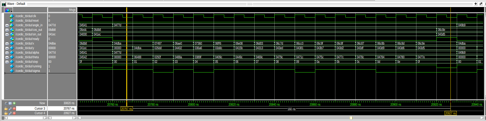
This can clearly be verified on the ModelSim timing diagram image here if you look at the time step 20760ns. You might want to click on the image to let it open in a separate tab and scroll around…
Notice how the value 0x0477d is in the angle_in and the alpha registers while 0x04dba and 0 are in the x and y registers.
Let’s now focus on the iterations proper. Notice how the step counter is at 0x00 for the full clock period between 20760 and 20770ns. The step counter will then count to 0x0f before the sin and cos are exposed as the valid answer at 20920ns.
The step counter hardware is synthesized properly in the FPGA because we told verilog that the counter should count up by a step of 1 (line 83) until 0x0f is reached (line 70). What happens between these lines, and as already presented above with the equations, is split in two main activities:
- rotating the internal vector
- tracking the value of theta while we chase the desired alpha
Rotating the internal vector
Let’s start with the rotation of the vector. Lines 75,76 or 80,81 told verilog to setup essentially the same computation tasks, albeit each one specialized in a single direction. We see x on line 75 being transformed by the optimized matrix rotation. In essence, we take the old value of x and add the value of y but bit shifted to the right by the value of step.
You can see the gradual rotation of the coordinates in the x and y traces on the timing diagram. Each step brings x and y closer to the expected answer values with decreasing adjustments as the shifting gets more intense with the step increase.
From a hardware perspective, both data paths for the positive and negative rotations were probably optimized into a single one with different settings, but the general idea remains that a full adder is at the center of all this. Being fed by either the full precedent value of itself and a selectively bit shifted version of either x and y. Are these being implemented as a real shift register or some bit field multiplexer? This could be validated by looking at the synthesis and placement reports. But one thing remains: the simulation with static timing runs the complete operation in one cycle at 100MHz without any perceived effort and the real FPGA runs the module at 50MHz without a glitch either.
Tracking the value of theta
The angle tracking is governed by the test at line 72 that will select the rotation direction based on the current value of theta compared to the desired angle.
Lines 74 and 79 add or subtract the actual angle imparted by the rotation using the precomputed values.
On the timing traces, we can clearly see how the initial theta of 0x0000 is gradually adjusted to match the value of alpha as close as possible: 0x477e instead of the desired 0x477d. Interestingly, the value of sigma has been traced to have a 1 representing a positive rotation and 0 for a negative rotation. We see how the algorithm used a series of positive and negative rotations to closely match the desired angle.
Performance
The algorithm, once translated into verilog and instantiated into a cyclone V FPGA, can easily produce 17 bit precision numbers within a packed 16+1 clock cycles pipeline. This means that a single cordic unit running at 50MHz can easily output the values within 170ns of being presented with an input. More than 5.8 million updates per second. The sin and cos errors are within an absolute error of 0.0002 and the concentricity error (Pythagorean length) is within 0.0004 units of the unit circle. That is 0.02% error on the sin or cos and 0.04% error on the concentricity.
Test and validation
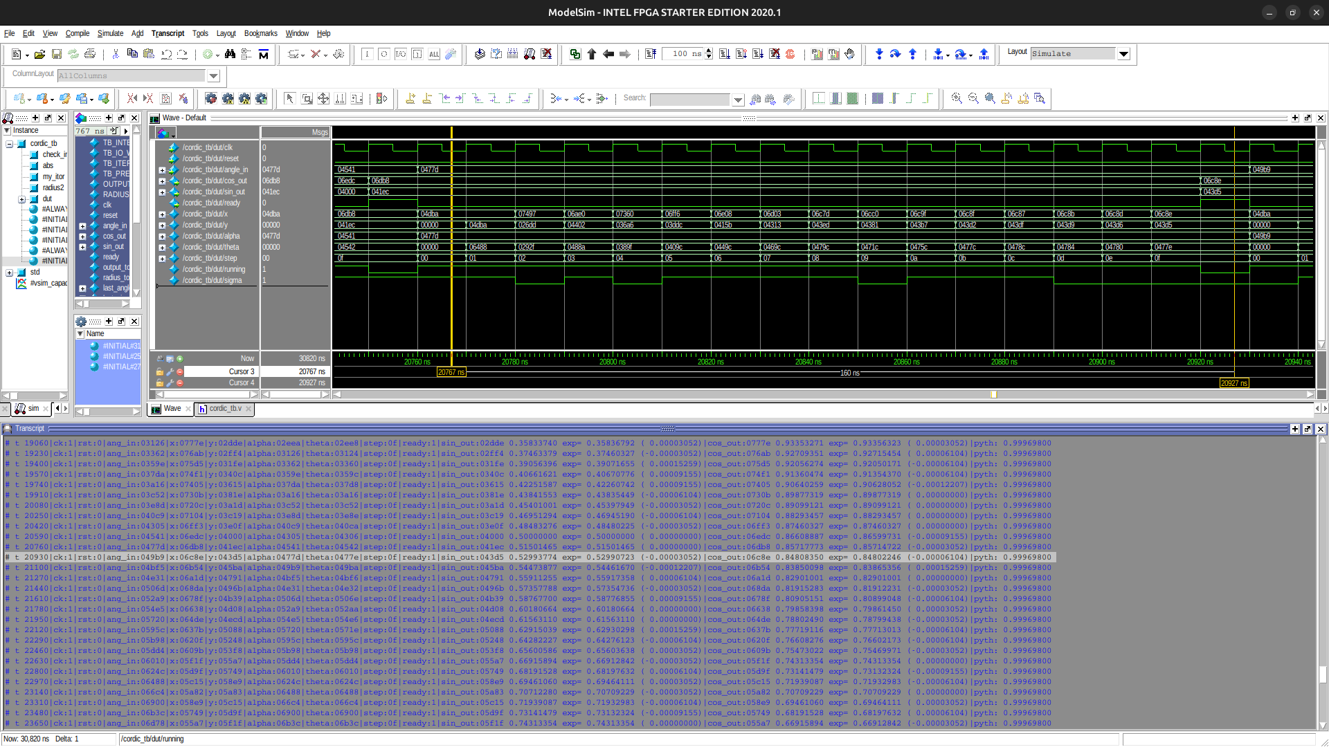
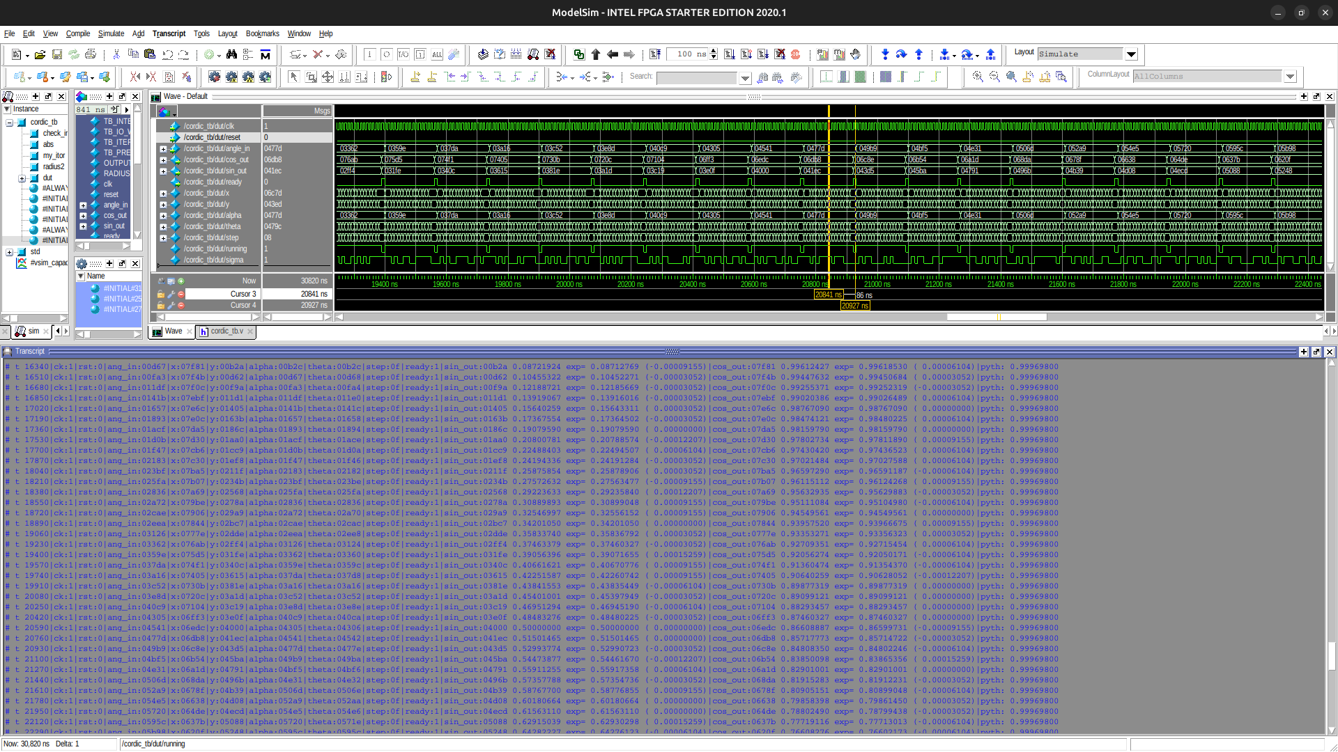
An test bench has been written as well as a set of accompanying C programs to validate the results and achieved resolution/precision. The programs also automatically precompute the fixed arctan table and the $K_{fixed}$ constants and has been implemented for the floating point theoretical version as well as for the fixed point integer, as implemented in HW, version.
On the stacked simulation images on the right, you can see some of the outputs of the test bench and the idea that all of the possible angles have been fed to the cordic in simulation to predict the performance and validate the proper values. Each output is tested for the expected value, the error and the Pythagorean norm error (eccentricity).
Leave me a message on my LinkedIn if you want to know more about this.
Conclusion
The thing works beautifully.
The algorithm, as designed, can also be extended to near arbitrary width and step sizes with regards to modern FPGAs. It consumes much less than 1% of the ressources of a cyclone V (5CGXFC5C6F27).
If you want to see the algorithm at work, please look into the project YouTube video where the roll input of the IMU is sent to this cordic to compute the cos and sin values used to rotate a bar graph in real time. Smooth!
Don’t forget to subscribe in the chat and comeback soon!